- Mon 12 November 2018
- brightway

Why would one calculate inventory flows?
In the beginning, there was nothing. Some stuff happened, and eventually life cycle analysis came into being. At first, we didn't have the tools to really translate inventory values into damages, so it wasn't quite life cycle assessment, but the characteristic equation looked quite similar:
The matrix B has dimensions biosphere flows (i.e. substances released to or consumed from air, water, soil) by activities, and f is a column vector, so the inventory is a column vector of biosphere flows.
However, sometimes we don't want biosphere flows, but technosphere flows, like the total amount of steel used to build a car.
Examining the supply array
We can get this information by manually examining the supply array (i.e. the solution to \(A^{-1}f\)):
STEEL_NAMES = {
    'steel production, converter, chromium steel 18/8',
    'steel production, converter, low-alloyed',
    'steel production, converter, unalloyed',
    'steel production, electric, chromium steel 18/8',
    'steel production, electric, low-alloyed',
    # Not actually production processes... ecoinvent ¯\_(ツ)_/¯
    #     'steel production, chromium steel 18/8, hot rolled',
    #     'steel production, low-alloyed, hot rolled',
    #     'reinforcing steel production',
}
STEELS = [x for x in bw.Database("ecoinvent 3.5 cutoff")
          if x['name'] in STEEL_NAMES]

car = next(x for x in bw.Database("ecoinvent 3.5 cutoff")
           if x['name'] == "passenger car production, petrol/natural gas")
lca = bw.LCA({car: 1000})  # Assume car is 1000 kilograms
lca.lci()
sum(lca.supply_array[lca.activity_dict[act.key]] for act in STEELS)

>>> 999.73
Note that I have done my best to find the activities that were actually steel production, as opposed to activities that already had steel as an input. However, it is certainly possible that I made some mistakes, and the numbers presented here may be inaccurate. The general conclusions should be valid, though.
Custom flows and LCIA methods
However, this isn't so elegant. Another way, and one that I prefer, is to add new biosphere flows for the quantities we are interested in. There are a couple reasons to prefer this approach:
- It fits into the standard LCA calculation framework for contribution analysis and graph traversal.
- It allows us to weight some quantities more than others - for example, instead of summing the total biomass, you could sum it's exergetic value, or each alloying element in each kind of steel.
- It can be easily shared with others, just like any other LCIA method.
On the other hand, it does require making modifications to the background database, which is normally avoided when possible.
We will create these new flows in a new database:
bw.Database("Inventory flows").write({
    ('Inventory flows', 'steel'): {
        'unit': 'kilogram',
        'type': 'inventory flow',
        'categories': ('inventory',),
    }
})
Add the new biosphere exchanges to our steel activities:
for act in STEELS:
    act.new_exchange(**{
        'input': ('Inventory flows', 'steel'),
        'type': 'biosphere',
        'amount': 1,  # Assumes production amount of 1
    }).save()
And finally, create a new LCIA method to assess steel flows:
m = bw.Method(("Inventory flows", "Steel"))
m.register(unit='kilogram')
m.write([
    (('Inventory flows', 'steel'), 1)
])
Now, calculating the steel required is just a normal LCA calculation:
lca = bw.LCA({car: 1}, ("Inventory flows", "Steel"))
lca.lci()
lca.lcia()
lca.score

>>> 999.73
Avoiding double counting
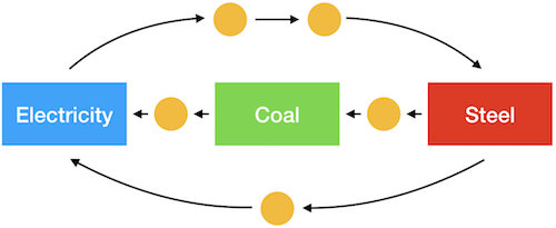
Imagine a system like the one above, where you wanted to calculate the steel needed for the electricity, coal, and steel production separately. Because there are loops in this graph, doing three separate calculations would lead to double counting: the steel for electricity would include the steel for the coal, but we also calculate the steel for the coal by itself. Similarly, demand for coal induces demand for electricity through steel production.
There are a number of ways to avoid double counting, including an approach that I wrote about earlier that uses Wurst to break these dependencies. However, this approach writes a complete new database, which is relatively expensive, especially done more than once. Instead, we can solve this problem by directly modifying the technosphere matrix.
A simplified example
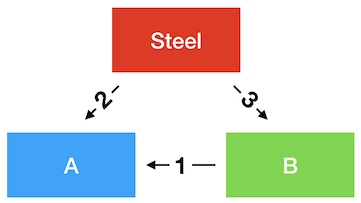
In this case, I hope we can all agree that to produce one unit of output from A, we need 5 units of steel.
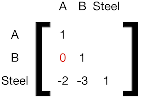
If we built a technosphere matrix, it would look like this:
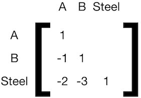
To be able to separate calculate the steel demand for A and B, we need to sever the connection between them:
To generalize this procedure, we use the following algorithm.
Given a set of activities for which we want to calculate separate material flows, \({activities}\), and a technosphere matrix \(A\), with rows \(i\) and columns \(j\), we can construct a new \(\hat{A}\) for each activity \(\alpha\) in \({activities}\):
Implementation in Brightway
Brightway exposes the relevant matrices, so this approach is relatively easy to implement:
def without_double_counting(lca, activity_of_interest, activities_to_exclude):
    """Calculate a new LCIA score for ``activity_of_interest`` but excluding
    contributions from ``activities_to_exclude``.

    * ``lca`` is an ``LCA`` object for which LCI and LCIA have already been calculated
    * ``activity_of_interest`` is a demand dictionary, e.g. {some_activity: amount}
    * ``activities_to_exclude`` is an iterable of activity objects or keys

    Returns the LCIA score.
    """
    assert hasattr(lca, "characterized_inventory"), "Must do LCI and LCIA first"

    tm_original = lca.technosphere_matrix.copy()

    to_key = lambda x: x if isinstance(x, tuple) else x.key

    exclude = set([to_key(o) for o in activities_to_exclude]).difference(
              set([to_key(o) for o in activity_of_interest]))

    for activity in exclude:
        row = lca.product_dict[activity]
        col = lca.activity_dict[activity]
        production_amount = lca.technosphere_matrix[row, col]
        lca.technosphere_matrix[row, :] *= 0
        lca.technosphere_matrix[row, col] = production_amount

    lca.redo_lcia(activity_of_interest)
    lca.technosphere_matrix = tm_original
    return lca.score
Example: Car components
We can apply our function to the car example calculated earlier. The two primary components in the car are the glider and the engine, and we want to know how much steel is in each of them, as well as how much residual steel is needed for everything else. We first calculate how much glider and engine we need for a 1000 kilogram car:
lca = bw.LCA({car: 1000}, ("Inventory flows", "Steel"))
lca.lci()
lca.lcia()

# market for glider, passenger car
glider = ('ecoinvent 3.5 cutoff', '3190a5aaecaaa169947d055586a0a4ae')

# market for internal combustion engine, passenger car
engine = ('ecoinvent 3.5 cutoff', 'e4bdb0c9a5612e4df90ac8c8cbc9692f')

for name, act in [("Glider", glider), ("Engine", engine)]:
    print(name, lca.supply_array[lca.activity_dict[act]])

>>> Glider 739.8802761540312
>>> Engine 260.1336051832947
We can then calculate the respective steel inputs in these three areas:
without_double_counting(lca, {car: 1000}, [glider, engine])
>>> 0.8322468900755811

without_double_counting(lca, {glider: 739.8802761540312}, [car, engine])
>>> 840.408990053158

without_double_counting(lca, {engine: 260.1336051832947}, [car, glider])
>>> 158.49646168629997
How can there be more than one kilogram of steel in one kilogram of glider?
According to ecoinvent 3.5, cutoff system model, one needs 1.136 kilograms of steel to make one kilogram of glider. How is this possible? One explanation could that there is steel needed in the various infrastructure elements used to make the glider, such as the factory, the iron ore mine, and the transportation grid. However, the main driver of this result is the cutoff system model, which "cuts off" credit for recycling. If we look into the processes used for glider production which have the highest steel losses (see the notebook for details), we see that we have losses in steel working activities, such as:
- steel production, chromium steel 18/8, hot rolled: 7.7% loss
- steel production, low-alloyed, hot rolled: 6.1%
It is the compounding of these losses that add up to 13.6%.
Of course, this steel does not just disappear - it is gathered, sorted, and recycled. But in the cutoff system model, there is no credit for producing recyclable materials, so they are removed from the supply chain graph. Ironically, this removal is mathematically the same as our procedure to avoid double counting. The cutoff model also has another somewhat ironic effect - a lot of our steel comes from electric arc furnaces, which are consuming recyclable iron scrap, which is itself cut off from iron production. Though we tend to use the cutoff system model as our default ecoinvent variant, it is clear that it is not a great choice when tracing material flows.
Example: Truck transport without light duty vehicles
Light duty vehicles (LDVs) have gross vehicle weights (i.e. the weight of the truck and its cargo) of less than 8 tons. They also have a different usage pattern than heavier trucks, as there are a number of service vehicles included in this weight class. Many models therefore separate light and heavy duty vehicles.
In ecoinvent, this weight class is labelled "3.5-7.5 ton."
We can see the steel input for all truck transport (measured in ton-kilometers), and separately for LDVs, following out pattern above:
trucks = next(x for x in bw.Database("ecoinvent 3.5 cutoff")
           if x['name'] == "market group for transport, freight, lorry, unspecified")
ldvs = [o for o in bw.Database("ecoinvent 3.5 cutoff")
        if o['name'].startswith("transport, freight, lorry") and "3.5-7.5 ton" in o['name']]
lca = bw.LCA({trucks: 1}, ("Inventory flows", "Steel"))  # 1 ton-kilometer
lca.lci()
lca.lcia()
print(lca.score)
>>> 0.0016023705343866921
lca.score - without_double_counting(lca, {trucks: 1}, ldvs)
>>> 2.168404344971009e-18
As expected, in this particular case the marginal steel input is quite small, as LDVs only contribute 3% of ton-kilometers, and have proportionately small amounts of truck mass.
Example: Demand for activities coming from an external model
We are currently working on providing steel and other inputs to the REMIND integrated assessment model (IAM). In this case, the numbers for total transport demand, electricity production, and other quantities come from the IAM, not from our examination of the supply chain. In this case, the calculations are actually even easier, as we can skip the step of looking up demands in the supply array. The only tricky thing is how to map REMIND demands to many ecoinvent activities. There are 76 lorry transport activities in ecoinvent, for example. Probably the most sensible approach is to take a weighted average using their production volumes, which are provided by ecoinvent:
def get_production_volume(act):
    return next(iter(act.production()))['production volume']
Here is an example calculation for 10.000 ton-kilometers of lorry transport and 100 kWh of electricity:
all_transport = {
    o: get_production_volume(o)
    for o in bw.Database("ecoinvent 3.5 cutoff")
    if o['name'].startswith("transport, freight, lorry")
}
total = sum(all_transport.values())
all_transport = {k: v / total * 1e4 for k, v in all_transport.items()}

all_electricity = {
    o: get_production_volume(o)
    for o in bw.Database("ecoinvent 3.5 cutoff")
    if o['name'].startswith("market for electricity,")
}
total = sum(all_electricity.values())
all_electricity = {k: v / total * 1e2 for k, v in all_electricity.items()}

without_double_counting(lca, all_transport, all_electricity)
>>> 0.001582994381059183
without_double_counting(lca, all_electricity, all_transport)
>>> 0.00216614294414289
Conclusions
The choice of ecoinvent system model plays a large role in material flow results. We (or, at least, I) need to think more about whether the allocation at point of substitution (APOS) system model would be adequate for material flow analysis, or if we need to develop a new system model.
We have previously used Wurst to create entirely new databases with the modifications we want. Here, we manipulate the technosphere matrix directly instead. Direct manipulation is more computationally efficient, but would not work well for some research questions. It is more transparent to have each type of manipulation isolated as a separate, testable function, and changes using Wurst can use additional metadata not otherwise available in the technosphere matrix. It can also be useful to have a copy of the modified database to share or inspect later. Though the research question and project audience will drive the ultimate choice of method, the availability of high-quality, flexible, and user-friendly open source LCA software is what makes such choices possible in the first place.