- Sun 03 August 2014
- brightway2
Performance has been one of the core values in Brightway2 since its creation almost two years ago. Some recent changes have made static LCA calculations in Brightway2 faster.
Finding the slow spots
Profiling is one of the key ways to test code speed. Here is the output from line_profiler for code that picks 10 random activities from ecoinvent 2.2:
  3082589 function calls (3079892 primitive calls) in 24.293 seconds

 ncalls  tottime  percall  cumtime  percall filename:lineno(function)
2719855   15.063    0.000   15.063    0.000 {method 'get' of 'dict' objects}
     23    2.640    0.115    2.640    0.115 {cPickle.load}
     10    2.141    0.214   19.896    1.990 matrices.py:181(build)
     40    1.880    0.047   17.243    0.431 fallbacks.py:7(indexer)
   3059    0.329    0.000    0.329    0.000 {numpy.core.multiarray.array}
     20    0.226    0.011    3.337    0.167 __init__.py:1(<module>)
     10    0.212    0.021    0.212    0.021 {__umfpack.umfpack_di_numeric}
     50    0.169    0.003    0.169    0.003 {method 'sort' of 'numpy.ndarray' objects}
     10    0.102    0.010    0.102    0.010 {__umfpack.umfpack_di_symbolic}
     34    0.072    0.002    0.093    0.003 {zip}
Normally, we would expect the library that actually solves the linear system of equations (umfpack) to take the most time, but in this case that is not true - it is loading the data from disk (cPickle.load), and then preparing that data ({method 'get' of 'dict' objects}, matrices.py:181(build), and fallbacks.py:7(indexer)) that takes the most time. If we look in detail at the build function in matrices.py, we can better understand exactly where the slow points are (you might have to scroll horizontally within the literal block below):
Total time: 20.2544 s

Line #      Hits         Time  Per Hit   % Time  Line Contents
==============================================================
   184                                               def build(cls, dirpath, names):
   185        10           46      4.6      0.0          assert isinstance(names, (tuple, list, set)), "names must be a list"
   186        10           16      1.6      0.0          array = load_arrays(
   187        10           10      1.0      0.0              dirpath,
   188        30        85551   2851.7      0.4              [Database(name).filename for name in names]
   189                                                   )
   (some comment lines removed)
   201        10           41      4.1      0.0          tech_array = array[
   202        10           22      2.2      0.0              np.hstack((
   203        10        11596   1159.6      0.1                  np.where(array['type'] == TYPE_DICTIONARY["technosphere"])[0],
   204        10       671236  67123.6      3.3                  np.where(array['type'] == TYPE_DICTIONARY["production"])[0]
   205                                                       ))
   206                                                   ]
   207        10           51      5.1      0.0          bio_array = array[np.where(
   208        10         9570    957.0      0.0              array['type'] == TYPE_DICTIONARY["biosphere"]
   209        10      1426665 142666.5      7.0          )[0]]
   210        10           73      7.3      0.0          tech_dict = cls.build_dictionary(np.hstack((
   211        10           47      4.7      0.0              tech_array['input'],
   212        10           16      1.6      0.0              tech_array['output'],
   213        10       162396  16239.6      0.8              bio_array['output']
   214                                                   )))
   215        10        57002   5700.2      0.3          bio_dict = cls.build_dictionary(bio_array["input"])
   216        10           60      6.0      0.0          cls.add_matrix_indices(tech_array['input'], tech_array['row'],
   217        10      2808268 280826.8     13.9                                 tech_dict)
   218        10           76      7.6      0.0          cls.add_matrix_indices(tech_array['output'], tech_array['col'],
   219        10      2800099 280009.9     13.8                                 tech_dict)
   220        10      6028841 602884.1     29.8          cls.add_matrix_indices(bio_array['input'], bio_array['row'], bio_dict)
   221        10      6064507 606450.7     29.9          cls.add_matrix_indices(bio_array['output'], bio_array['col'], tech_dict)
   222        10        51402   5140.2      0.3          technosphere = cls.build_technosphere_matrix(tech_array, tech_dict)
   223        10        76750   7675.0      0.4          biosphere = cls.build_matrix(bio_array, bio_dict, tech_dict, "row", "col", "amount")
   224        10           24      2.4      0.0          return bio_array, tech_array, bio_dict, tech_dict, biosphere, \
   225        10           12      1.2      0.0              technosphere
The vast majority of the time is spend on the function cls.add_matrix_indices. What is this function, and what does it do? Luckily, the new, consolidated Brightway2 manual explains this in detail. The reason it is so slow is that add_matrix_indices is written in pure Python. With the help of two libraries, we can make this much faster. First, we write a different version of add_matrix_indices in Cython. Cython is essentially Python with static types, at least in this case. This new module is called bw2speedups. The actual Cython code is not that different from pure Python code, but the performance difference is astounding. However, Cython code doesn't help people who don't have a C compiler on their computer, and most OS X and Windows users don't. The second library is a new Python packaging standard called wheel, which allows compiled code to be easily made available on the Python package index. After some pain and suffering, I have compiled bw2speedups for OS X 10.7, 10.8, and 10.9, and for both the 32- and 64-bit versions of Windows >= 7.
But let's not stop there - what about lines 204 and 209? That is another slow point. In these lines, we have a single array of values, and take values to make the technosphere or biosphere matrices based on the value in the column type. This code uses NumPy "fancy indexing", where you can pass in an array of indices to get a new array with only those rows, i.e.
In [1]: import numpy as np

In [2]: arr = np.arange(100, 110)

In [3]: indices = np.random.randint(0, 10, size=5)

In [4]: arr
Out[4]: array([100, 101, 102, 103, 104, 105, 106, 107, 108, 109])

In [5]: indices
Out[5]: array([8, 8, 6, 1, 7])

In [6]: arr[indices]
Out[6]: array([108, 108, 106, 101, 107])
It turns out that using the NumPy function take is much faster than fancy indexing, even though they are doing the same thing:
In [1]: import numpy as np

In [2]: arr = np.arange(100000)

In [3]: indices = np.random.randint(0, 100000, size=50000)

In [4]: %timeit arr[indices]
1000 loops, best of 3: 470 µs per loop

In [5]: %timeit arr.take(indices)
1000 loops, best of 3: 228 µs per loop
When we apply both these changes, and re-run our profiling code, this is what we get:
 364736 function calls (362039 primitive calls) in 4.324 seconds

ncalls  tottime  percall  cumtime  percall filename:lineno(function)
    23    2.685    0.117    2.685    0.117 {cPickle.load}
    40    0.368    0.009    0.368    0.009 {bw2speedups._indexer.indexer}
    10    0.211    0.021    0.211    0.021 {__umfpack.umfpack_di_numeric}
    10    0.105    0.011    0.105    0.011 {__umfpack.umfpack_di_symbolic}
    50    0.094    0.002    0.094    0.002 {method 'sort' of 'numpy.ndarray' objects}
    34    0.071    0.002    0.092    0.003 {zip}
    20    0.060    0.003    0.060    0.003 {scipy.sparse._sparsetools.csr_sort_indices}
   205    0.029    0.000    0.075    0.000 doccer.py:12(docformat)
    20    0.024    0.001    0.024    0.001 {method 'take' of 'numpy.ndarray' objects}
    10    0.022    0.002    0.022    0.002 {__umfpack.umfpack_di_solve}
The major consumer of time is now loading our data from disk, but this is already a C library (cPickle), and is quite efficient. The next lines are either the function we rewrote in Cython (bw2speedups._indexer.indexer), or the umfpack numerical algorithms; in both cases, we don't really have a chance of making them faster.
How much faster?
So how much faster is an LCA calculation with these two changes? Here are the total times in seconds needed for a single LCA calculation on a nice 2011 laptop, for both ecoinvent 2.2 and 3.1 cutoff, with the base case and our two changes:
| Database | Base case | With bw2speedups | With bw2speedups and numpy.take |
|---|---|---|---|
| Ecoinvent 2.2 | 1.92 | 0.314 | 0.120 |
| Ecoinvent 3.1 cutoff | 7.22 | 1.28 | 0.535 |
Single static LCA calculations are now 10 times faster! These times also compare quite well with the competition.
Getting the new code
Read the manual section on upgrading Brightway2, and then run the following:
pip install bw2speedups
pip install -U --no-deps bw2calc
Multiple calculations for the same database
When we are assessing multiple functional units from the same database, we can factorize the technosphere matrix. This will take more time at the beginning, but will make future calculation much faster. The normal inventory calculation code is:
from brightway2 import *
lca = LCA({Database("ecoinvent 2.2").random(): 1})
lca.lci()
Versus the factorized call:
from brightway2 import *
lca = LCA({Database("ecoinvent 2.2").random(): 1})
lca.lci(factorize=True)
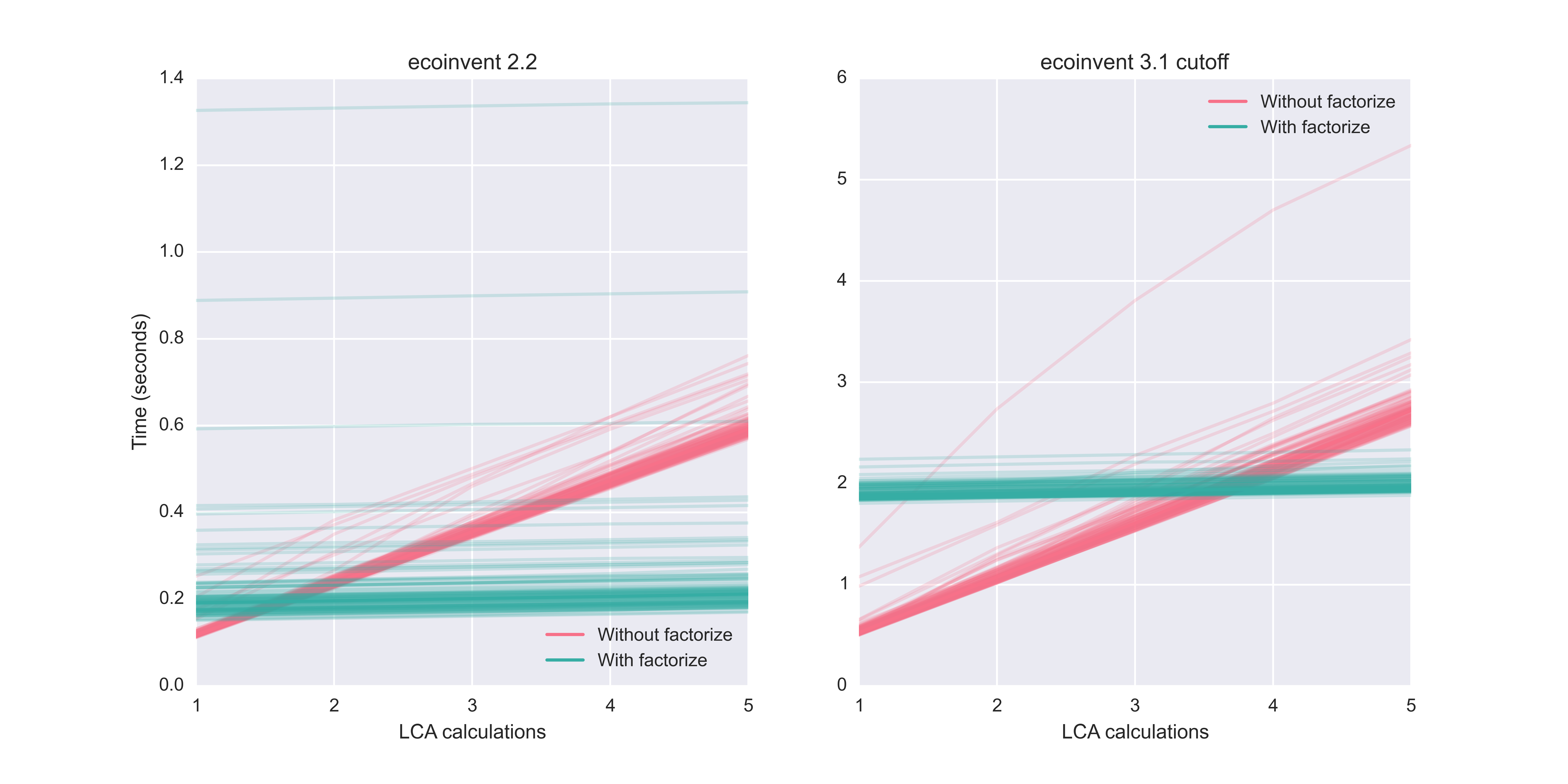
We can investigate when factorization is worthwhile by using the LCA.redo_lci function, and graphing the total time for both factorized and non-factorized calculations. We do this 100 times for each possibility to get a representative sample of possible times:

Calculation times for multiple functional units drawn from ecoinvent 2.2 and 3.1 cutoff
For ecoinvent 2.2, factorization is worthwhile when doing even two calculations from the same database. For 3.1 cutoff, the initial factorization penalty is bigger, and the break-even point is four calculations. However, as a general rule, factorize when doing multiple calculations, and don't bother for a single calculation.
Monte Carlo calculations
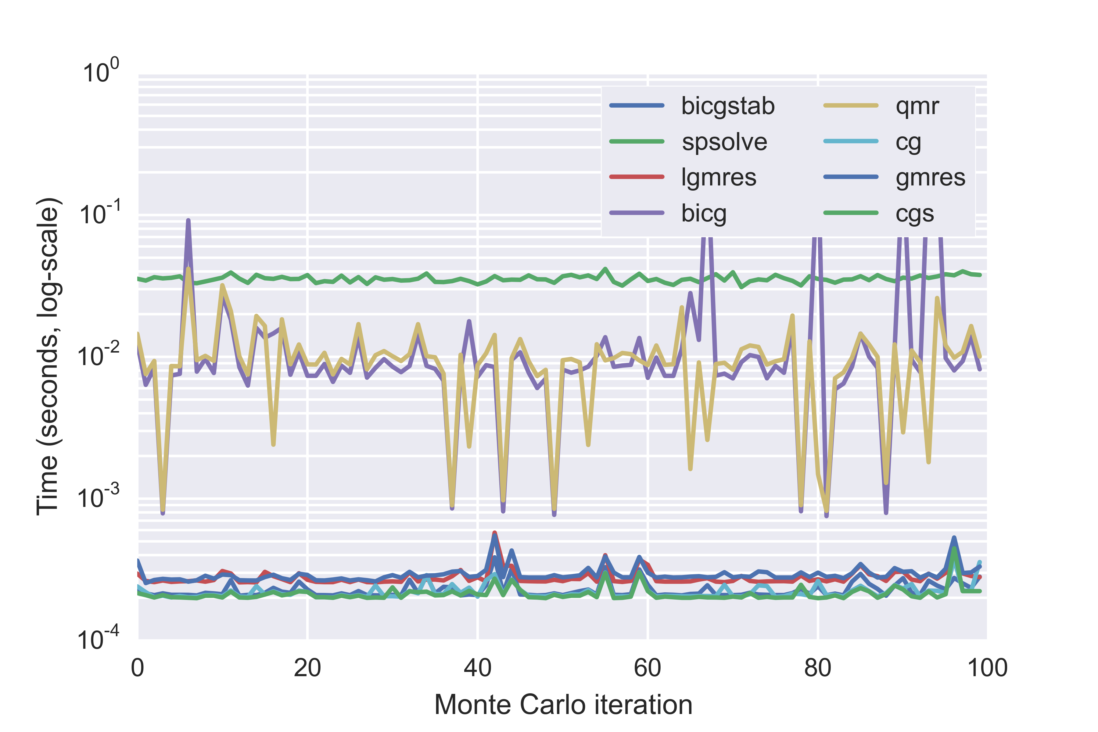
With Monte Carlo calculations, we can use another trick to make calculations quick. We can't factorize the technosphere matrix, because it changes with each Monte Carlo iteration. But we are assessing the same functional unit each time, which means we can use the supply vector calculated from the first Monte Carlo iteration as an initial guess for the supply vector for each subsequent calculation, and use sparse iterative solvers. The speed advantage of iterative solvers is huge - up to two orders of magnitude. In the following figure, I tested seven iterative solvers, as well as the normal UMFpack direct solver (spsolve in the graph), for 100 Monte Carlo iterations, using a different activity from ecoinvent 2.2 each time. To make the comparison fair, I used the same activity and Monte Carlo sample data for each solver method. Note that this graph should have points instead of lines, as each iteration is independent of other iterations, but points are difficult to see.

Calculation times for seven iterative methods and the UMFpack direct solver (spsolve) for 100 Monte Carlo iterations
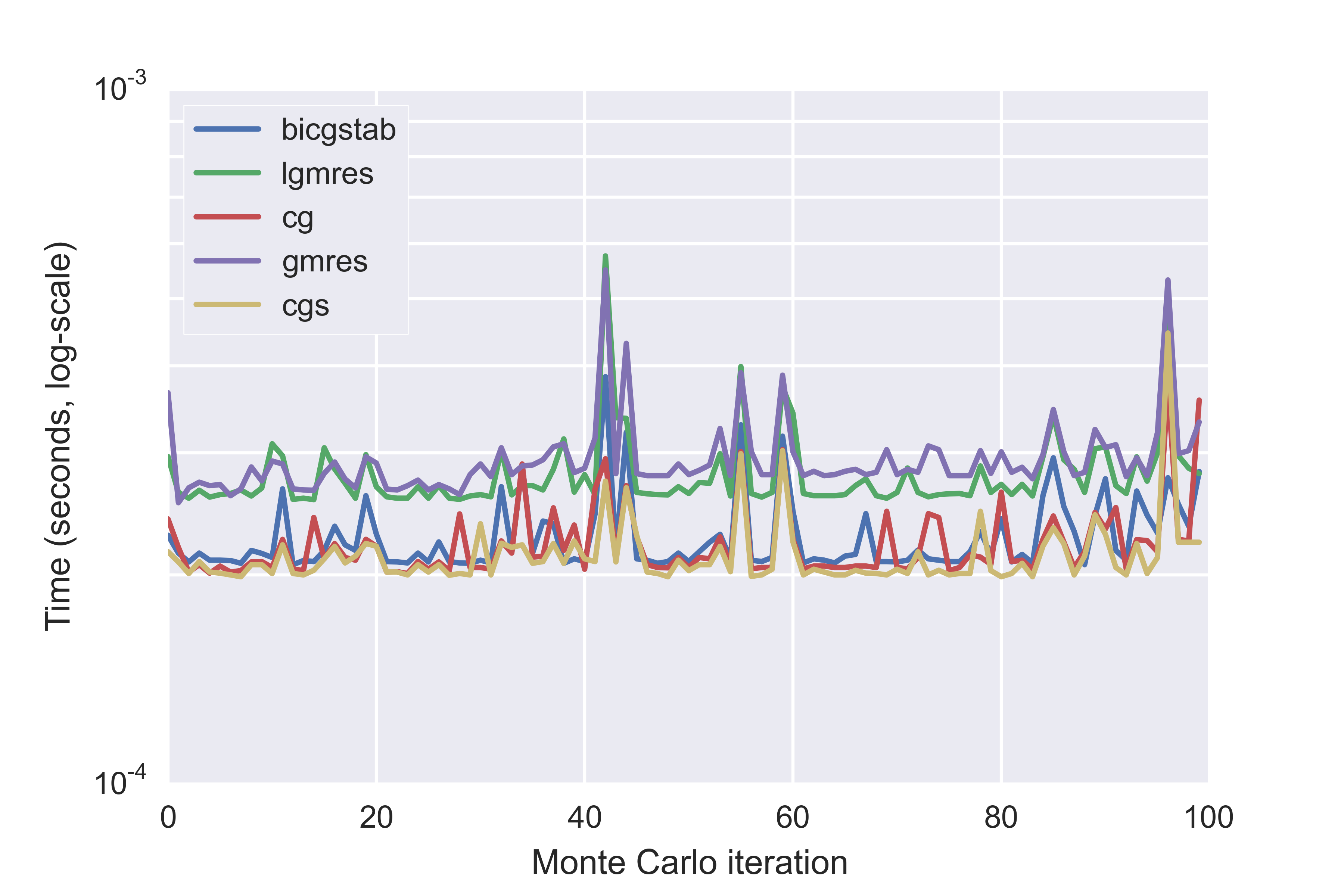
If we exclude the direct solver, and two slower methods, we can see the differences between the faster iterative methods in more detail:

Calculation times for the five fastest iterative solvers for 100 Monte Carlo iterations
The default solver in Brightway2 is cgs, which also has the lower average time. cgs is conjugate gradient squared - you can read about the various techniques in the scipy documentation or elsewhere. The difference between cgs (conjugate gradient squared), cg (conjugate gradient), and bicgstab (biconjugate gradient stabilized) is, however, rather small.
The performance of iterative solvers depends on how accurate the initial guess is, and this in turn depends on how much uncertainty is in the technosphere matrix. The cases where the supply vector differed substantially from the initial guess show up as spikes in calculation time, as more work is required to converge on the new supply vector. This difference would also show up as a substantially different LCIA score.
| Solver | Minimum | Average | Maximum |
|---|---|---|---|
| cgs | 0.00020 | 0.00021 | 0.00045 |
| cg | 0.00020 | 0.00022 | 0.00038 |
| bicgstab | 0.00021 | 0.00023 | 0.00039 |
| lgmres | 0.00026 | 0.00028 | 0.00058 |
| gmres | 0.00025 | 0.00029 | 0.00055 |
| qmr | 0.00082 | 0.01018 | 0.04179 |
| bicg | 0.00075 | 0.02279 | 0.27846 |
| spsolve | 0.03102 | 0.03553 | 0.04168 |
Ecoinvent 3.1
The sad truth is that the uncertainty values in ecoinvent 3.1 are much too high, and in my opinion, they were not reviewed in sufficient detail. For example, there is only activity dataset with an exchange that has a listed lognormal sigma (roughly equivalent to a standard deviation) of $1.98 \cdot 10^{138}$, i.e. 2 follow by over 100 zeros, i.e. a big number. This dataset was reviewed and approved by two people at the ecoinvent centre.
In addition to being obviously incorrect, these large values for uncertainties mean that each Monte Carlo iteration will have a supply vector that is substantially different from iteration to iteration. These large differences make the iterative solvers have very poor performance.
Conclusions
- Install bw2speedups and version 0.16 of bw2calc to get a ten-fold increase in LCA calculation performance.
- Factorize the technosphere matrix if you are going to do repeated calculations from the same database, but don't bother if only doing one calculation.
- Use one of the conjugate gradient iterative solvers for Monte Carlo calculations.
- Ecoinvent version 3.1 is not yet ready for uncertainty analysis.
