Building the matrices

We will assume that we are modelling a linear system, i.e. one where there are strict linear relationships between inputs and outputs, and where each production function can supply an infinite amount of its reference product. These are assumptions which don't hold in the real world, but are relatively standard in life cycle assessment.

Let's imagine a very simple system - the production of a steel bicycle. In our example system we can write two equations, one each for the production of the bicycle and the production of the steel tubes used to make the bicycle. We can write the equations however we want, but in this case we will use the convention that inputs are on the left and outputs on the right:

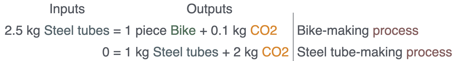
CO2 is an output - it's emitted by the processes. The steel tubes come for free because we are making the example simple.

Let's see what happens if we move everything over to the right hand side:

Here we have already discovered a very important concept - we will have positive and negative numbers in our equations, and therefore we need a sign convention that is applied consistently and that we can understand. Brightway uses the following sign convention:

• Products which are consumed have a negative number
• Products which are produced have a positive number
• Elementary flows are special

Traditionally elementary flows have an environmental context - something like emissions to air or natural resources. The implication of this tradition is that, in some contexts (like natural resources), elementary flows being consumed are positive, while in other contexts (like emissions to air) elementary flows being released are also positive. This tradition is the exact opposite of how we treat products, but because it is followed by all inventory databases and impact assessment methods that I know of (characterization factors are positive, even if they are characterizing resource consumption), it is easier to follow this convention than risk introducing errors by changing numbers.

It would be nicer to have a single consistent sign convention.

Because we are modelling this as a linear system, we can put these coefficients into a matrix. Brightway also has a convention here: processes are columns, and products or elementary flows are rows.

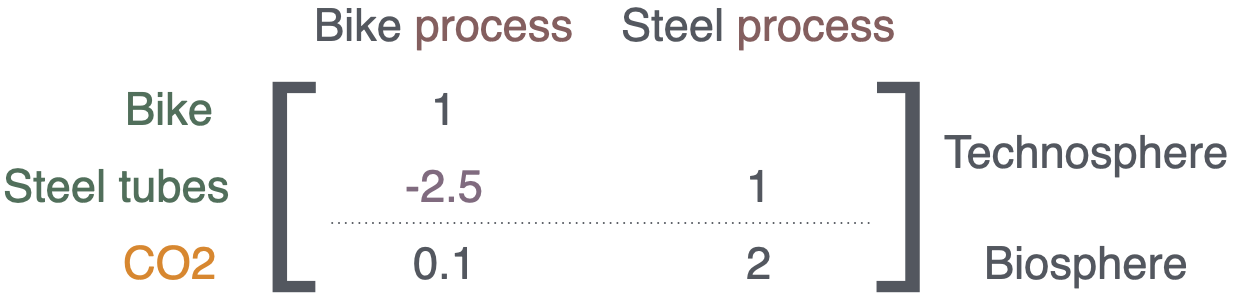
We don't have to put zeros in places where we don't have data - we will be building a sparse matrix, where empty elements are assumed to be zero.

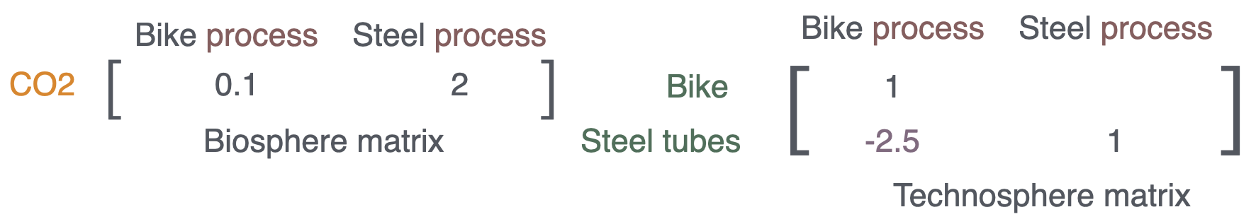
However, we can't use this equation to solve \(\textbf{A}x=f\) because our matrix isn't square - it has three rows and two columns. Instead, we can split this matrix into two different matrices. Brightway calls these the technosphere and the biosphere matrices:

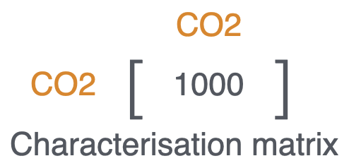
If we want to do impact assessment, then we also need a characterization matrix. This matrix turns the physical elementary flows into whatever unit of damage the impact category is describing - for example, Comparative Toxic Units instead of kilograms. This characterization matrix, \(\textbf{C}\), has both rows and columns of elementary flows, and only has numbers on its diagonal. Each number in the characterization matrix is, like everything else, a linear coefficient.

We have a lot of the number 1 already - let's do characterization in grams of CO2-equivalent. Our characterization factor would therefore be 1000 gram CO2-equivalent per kg of CO2:

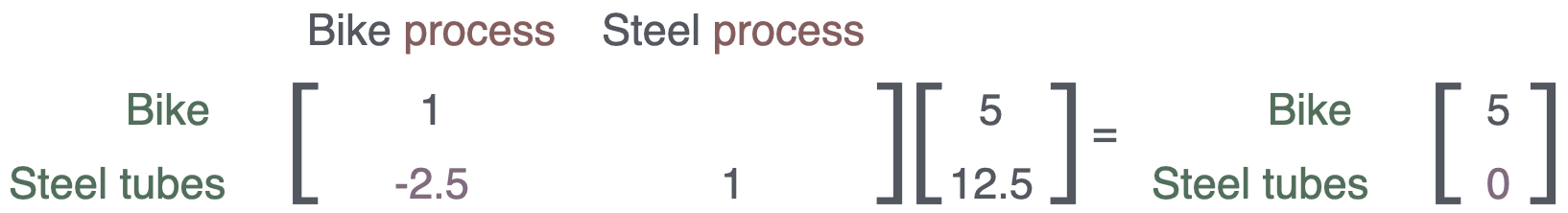
Before we figure out how to build this system in Brightway, let's look at how we could solve this simple system manually. Our technosphere matrix is the \(\textbf{A}\) in \(\textbf{A}x=f\) - what are the other values? \(f\) is the demand array, which specifies how much of each possible product we want, and \(x\) is the supply array - the amount of each process needed to supply the demand, and the result of solving \(\textbf{A}x=f\). We don't know \(x\) until we do some math, but we get to choose \(f\). Let's do a calculation for 5 bikes and nothing else. We would then have:

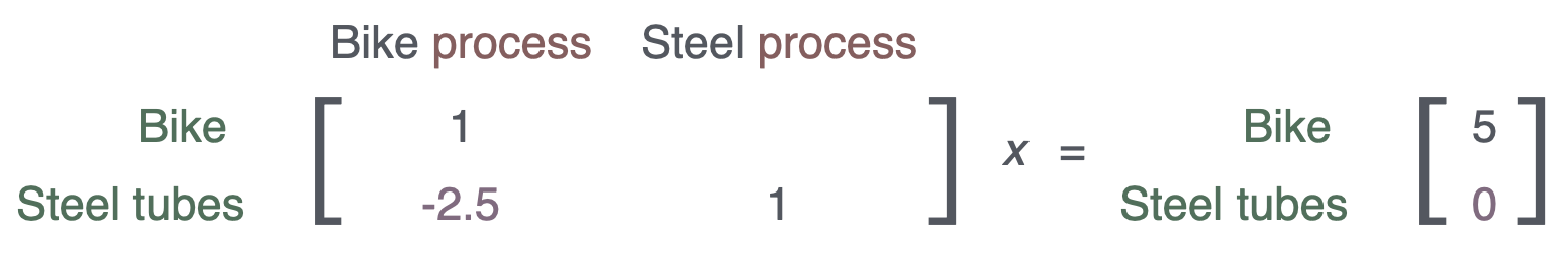
What values do we need in \(x\) to satisfy our demand? If we start with the first row, we can see that we need to scale the bike making process by 5 to get enough bike product to meet the demand. Our first value in \(x\) is therefore 5.

We now have a problem - our demand vector doesn't ask for any steel tube production, but by scaling the bike production by 5, we now have -12.5 (note the negative) kilograms of steel tube, not zero kilograms. We can now scale the steel tube process up to produce enough steel tubes to cancel out this negative number. The scaling factor is 12.5, because each time the steel tube making process is run it produces 1 kilogram of steel tubes. We have now solved our linear system and can put in the correct values for \(x\):

Humans make lots of mistakes, so let's put this data in the computer and make sure we have the right answer. We will start with a dense Numpy array first:

import numpy as np
A = np.array([
    (1,    0),
    (-2.5, 1)
])
f = np.array((5, 0))
np.linalg.solve(A, f)
>>> array([ 5. , 12.5])

The solvers we will use do something similar, but use tricks to make it possible to solve very large systems quickly.

The induced scaling of the steel-making process is also how substitution works - if we had a process which produced two products (two positive numbers), but our demand was only for one of them, then another process would have to decrease (have a negative scaling factor) to zero out the production of the second good. That's why there is no mathematical difference between production and substitution - we just use different labels to show the intent of the modeller.

In real practice, we will have large and pretty sparse technosphere matrices, so let's see how this would work with a Scipy sparse matrix instead of a dense Numpy array. This will require a bit more work - Brightway uses the constructor from Scipy which looks like this:

from scipy.sparse import csr_matrix
csr_matrix((data, (row_ind, col_ind)), [shape=(M, N)])

Where:

• data is a 1-d Numpy array with the non-zero elements in the technosphere matrix
• row_ind is a 1-d Numpy array in the same order as data; row_ind[x] give the row index of data[x].
• col_ind is a 1-d Numpy array in the same order as data; col_ind[x] give the column index of data[x].
• (M, N) are the number of rows and columns in the matrix. Because we don't specify values of zero, the matrix could be larger than the rows and columns given in the preceding arrays if there are columns or rows completely filled with zeros.

The row_ind and col_ind can be confusing. They are all one-dimensional, and have the same length. The way I remember how it works is: if element 7 of data is 3.141, element 7 of row_ind is 11, and element 7 of col_ind is 56, then we know that in row 11 and column 56 of the matrix being built there will be a value of 3.141.

The CSR sparse matrix constructor has a very nice property - you can specify multiple values for the same matrix element, and these values will be added together. In the LCA context, this means we can specify that a given process produces one kilogram of product, but also loses a small amount due to spoilage, and the matrix constructor will automatically give us the correct net production amount.

import numpy as np
from scipy.sparse import csr_matrix

data = np.array([1, -0.1])
row_ind = np.array([0, 0])
col_ind = np.array([0, 0])
shape = (1, 1)
matrix = csr_matrix((data, (row_ind, col_ind)), shape=shape)
matrix.todense()
>>> matrix([[0.9]])

In our example, our data array would have three values - the non-zero elements of the matrix. The row and column indices should be in the same order as the data, and keep in mind that Python starts indices with zero. So our first non-zero value is 1, in row 0 (we start counting with zero) and column 0. The next is -2.5, in row 1 and column 0. Finally, we have the data value 1, in row 1 and column 1:

import numpy as np
from scipy.sparse import csr_matrix

data = np.array([1, -2.5, 1])
row_ind = np.array([0, 1, 1])
col_ind = np.array([0, 0, 1])
shape = (2, 2)
matrix = csr_matrix((data, (row_ind, col_ind)), shape=shape)
matrix.todense()
>>> matrix([[ 1. ,  0. ],
>>>         [-2.5,  1. ]])

The best sparse solver depends on your CPU architecture. If you don't have the best solver for your CPU, Brightway will let you know:

from bw2calc import spsolve
>>> It seems like you have an ARM architecture, but haven't installed scikit-umfpack:
>>>
>>>     https://pypi.org/project/scikit-umfpack/
>>>
>>> Installing it could give you much faster calculations.
>>>
>>>   warnings.warn(UMFPACK_WARNING)

We can then use the solver to solve our linear problem:

from bw2calc import spsolve
spsolve(matrix, b)
>>> array([ 5. , 12.5])

from bw2data.snowflake_ids import snowflake_id_generator
next(snowflake_id_generator)
>>> 169741598115975168

from matrix_utils import ArrayMapper
import numpy as np

bike_making = 555555555
steel_tube_making = 666666666
bike = 123456789
steel_tubes = 111111
CO2 = 1

am = ArrayMapper(array=np.array([bike_making, steel_tube_making, bike, steel_tubes, CO2]))
am.map_array(np.array([steel_tubes, bike]))
>>> array([1, 2])

from matrix_utils import ArrayMapper
from scipy.sparse import csr_matrix
import numpy as np

bike_making = 555_555_555
steel_tube_making = 666_666_666
bike = 123_456_789
steel_tubes = 111_111
CO2 = 1

process_mapper = ArrayMapper(array=np.array([bike_making, steel_tube_making]))
product_mapper = ArrayMapper(array=np.array([steel_tubes, bike]))
biosphere_mapper = ArrayMapper(array=np.array([CO2]))

data = np.array([1, -2.5, 1])
row_ind = product_mapper.map_array(np.array([bike, steel_tubes, steel_tubes]))
col_ind = process_mapper.map_array(np.array([bike_making, bike_making, steel_tube_making]))
shape = (2, 2)
technosphere_matrix = csr_matrix((data, (row_ind, col_ind)), shape=shape)
technosphere_matrix.todense()

>>> matrix([[-2.5,  1. ],
>>>         [ 1. ,  0. ]])

from matrix_utils import ArrayMapper
from scipy.sparse import csr_matrix
import numpy as np

bike_making = 555_555_555
steel_tube_making = 666_666_666
CO2 = 1

process_mapper = ArrayMapper(array=np.array([bike_making, steel_tube_making]))
biosphere_mapper = ArrayMapper(array=np.array([CO2]))

data = np.array([0.1, 2])
row_ind = biosphere_mapper.map_array(np.array([CO2, CO2]))
col_ind = process_mapper.map_array(np.array([bike_making, steel_tube_making]))
shape = (1, 2)
biosphere_matrix = csr_matrix((data, (row_ind, col_ind)), shape=shape)

data = np.array([1000])
only_ind = biosphere_mapper.map_array(np.array([CO2]))
shape = (1, 1)
characterization_matrix = csr_matrix((data, (only_ind, only_ind)), shape=shape)

biosphere_matrix.todense(), characterization_matrix.todense()
>>> (matrix([[0.1, 2. ]]), matrix([[1000]]))

bike_index = product_mapper.map_array(np.array([bike]))

f = np.zeros(2)
f[bike_index] = 5

characterization_matrix @ biosphere_matrix @ spsolve(technosphere_matrix, f)
>>> array([25500.])

Datapackages: Persisting Matrix Data

It would be nicer if we had all this data in a prepared form, so we didn't need to build the mappers, arrays, etc. every time. The Brightway library bw_processing does exactly that: it defines a standard way of storing this data so it can be easily loaded into a matrix builder and used in calculations.

These bw_processing datapackages are based on the frictionless data datapackage standard, which defines how to attach data resources, and how to include and serialize metadata.

Let's put the data we have into a datapackage and use it in a calculation. First, we create an in-memory datapackage. bw_processing uses fsspec, which allows file storage on many kinds of filesystems, but in-memory is OK for now.

Next, we need to add the data to the datapackage. Because our libraries are designed to work together, it is relatively easy. The only major difference with what we did before is that we can glue the row and column indices together in one array - they are always in the same order and only used together, and so there is no reason to keep them separate.

We do this gluing by creating a Numpy record array - a special kind of array where each row is defined by a tuple of (label, datatype) pairs. In our case it looks like this:

import bw_processing as bwp
bwp.INDICES_DTYPE
>>>[('row', numpy.int64), ('col', numpy.int64)]

This data is coming from the database, and uses database ids. We wouldn't want to map it to matrix indices in any case as we don't know what other background databases will be used, which means we don't know the size of the matrices or anything else about them yet.

Datapackages can include multiple resource groups, though all datapackages produced by Brightway will only include either inventory or impact assessment data. In this example we can put everything into a single datapackage:

import bw_processing as bwp

technosphere_indices = np.array([
    # row, column
    (bike, bike_making),
    (steel_tubes, bike_making),
    (steel_tubes, steel_tube_making)
], dtype=bwp.INDICES_DTYPE)
technosphere_data = np.array([1, -2.5, 1])

dp = bwp.create_datapackage()
dp.add_persistent_vector(
    matrix="technosphere_matrix",
    indices_array=technosphere_indices,
    data_array=technosphere_data
)

biosphere_indices = np.array([
    (CO2, bike_making),
    (CO2, steel_tube_making),
], dtype=bwp.INDICES_DTYPE)
biosphere_data = np.array([0.1, 2])
dp.add_persistent_vector(
    matrix="biosphere_matrix",
    indices_array=biosphere_indices,
    data_array=biosphere_data
)

characterization_indices = np.array([
    (CO2, CO2),
], dtype=bwp.INDICES_DTYPE)
characterization_data = np.array([1000.])
dp.add_persistent_vector(
    matrix="characterization_matrix",
    indices_array=characterization_indices,
    data_array=characterization_data
)

You can see all the available information about one of the resource groups with:

next(group.metadata for _, group in dp.groups.items())

There is quite a lot!

{'profile': 'data-package',
 'name': 'd54118b9a0c64009aefe82cf10b46771',
 'id': 'ede8cb8ccf134732af7be138c07bbced',
 'licenses': [{'name': 'ODC-PDDL-1.0',
   'path': 'http://opendatacommons.org/licenses/pddl/',
   'title': 'Open Data Commons Public Domain Dedication and License v1.0'}],
 'created': '2025-04-10T20:35:11.305245+00:00Z',
 'combinatorial': False,
 'sequential': False,
 'seed': None,
 '64_bit_indices': True,
 'sum_intra_duplicates': True,
 'sum_inter_duplicates': False,
 'matrix_serialize_format_type': 'numpy',
 'resources': [{'profile': 'data-resource',
   'format': 'npy',
   'mediatype': 'application/octet-stream',
   'name': 'd9fc130dcfc6464e929950b56a0498d1.indices',
   'matrix': 'technosphere_matrix',
   'kind': 'indices',
   'path': 'd9fc130dcfc6464e929950b56a0498d1.indices.npy',
   'group': 'd9fc130dcfc6464e929950b56a0498d1',
   'category': 'vector',
   'nrows': 3},
  {'profile': 'data-resource',
   'format': 'npy',
   'mediatype': 'application/octet-stream',
   'name': 'd9fc130dcfc6464e929950b56a0498d1.data',
   'matrix': 'technosphere_matrix',
   'kind': 'data',
   'path': 'd9fc130dcfc6464e929950b56a0498d1.data.npy',
   'group': 'd9fc130dcfc6464e929950b56a0498d1',
   'category': 'vector',
   'nrows': 3}]}

This single datapackage is all we need to do an LCA calculation:

import bw2calc as bc

lca = bc.LCA(demand={bike: 5}, data_objs=[dp])
lca.lci()
lca.lcia()
lca.score
>>> 25500.0

In normal Brightway usage we wouldn't start with an in-memory datapackage, but one which has already been written to the local filesystem. Let's trace the code flow on how Brightway would do this calculation given a functional unit and an impact category from the database.

First, Brightway would look up the datapackages it needs for the given calculation. This includes looking at the dependent datapackages needed for the functional unit (e.g. if you built your foreground data on top of Exiobase, this would be two different datapackages), as well as the datapackages for the impact category. A normal Brightway calculation would have between three and ten datapackages loaded.

The bw2calc library will call the matrix_utils library to create MappedMatrix instances from the datapackages for each matrix needed for the given calculation. The MappedMatrix class creates and stores the information needed to go from database ids to matrix indices (the ArrayMapper that we saw earlier), and makes sure that these are used consistently for all datapackages and matrices - the order of processes in the technosphere and biosphere matrices must be the same.

MappedMatrix also allows for some functionality we won't discuss in this post, including specifying custom indexers, RNG seeds, dynamic matrix values, combinatorial sampling, and possibility arrays. See the bw_processing documentation for details on this functionality.

We also need to borrow the product mapper from the technosphere matrix to correctly create the demand array.

Finally, Brightway doesn't actually calculate \(h = CBA^{-1}f\), because this collapses the result matrix to a single score. It can be quite helpful to instead look at the characterized inventory matrix, which has rows of elementary flows and columns of processes. Therefore we use this alternative equation:

This gives us a characterized inventory result matrix with rows of elementary flows and columns of processes - the same form as the life cycle inventory matrix.

lca.characterized_inventory.todense()
>>> matrix([[  500., 25000.]])

With the characterized inventory matrix, we can sum and sort all the columns to find the most damaging elementary flow (in the example it's CO2, there is only one elementary flow 😊), but we can do the same to the rows to find the most damaging process:

process_indices_by_damage = np.argsort(
    np.abs(
        lca.characterized_inventory.sum(axis=0).data
    ).ravel()
)[::-1]

[lca.dicts.activity.reversed[index] for index in process_indices_by_damage]
>>> [666666666, 555555555]

This returns the database ids we defined earlier. and the order is what we would expect given that we know steel tube making (666666666) emits more CO2 than bike making (555555555).

Brightway supports a variety of uncertainty, scenario, and variant analyses, but they all boil down to the same mathematical trick - we want to change one or matrices by using different versions of the data vector, but leaving the indices the same. There is a lot of flexibility on how this is implemented, depending on whether the set of possible values in known in advance or generated dynamically, and the degree of value correlation across matrices (see for example this and this).

That's basically bw2calc and its support libraries. Let's turn to how Brightway stores data in a database.

Graph Database

At is core, bw2data is a wrapper around SQLite used as a graph database, plus some metadata storage in JSON files. We have two main tables, one for nodes (currently called activitydataset) and the other for edges (currently called exchangedataset). Nodes are products, processes (including multifunctional processes), and elementary flow objects; Edges are directed qualitative or quantitative relationships between nodes.

Brightway's data model for edges kind of looks like the following. It isn't exactly this, but you should think of it like this:

from dataclasses import dataclass

@dataclass
class Edge:
    target: int  # database id
    source: int  # database id
    data: dict

Similarly, you should think of nodes as following this simple data model:

from dataclasses import dataclass
from enum import StrEnum

@dataclass
class Node:
    id: int
    type: StrEnum
    collection: str
    data: dict

Nodes belong to collections, which are containers to store metadata about a number of nodes associated together. For example, the US LCA commons is a container for process and product nodes, and refers to the fedelemflowlist, a collection of elementary flows.

Brightway uses different kinds of collections for inventory and impact assessment data. However, they all roughly follow this simplified data model:

from dataclasses import dataclass
from datetime import datetime
from typing import Any

@dataclass
class Collection:
    id: Any
    modified: datetime
    data: dict

The datapackages needed for bw2calc map one-to-one with collections in bw2data. In standard LCA, there are only two types: inventory database datapackages and impact category datapackages. Extensions like regionalization or the inclusion of normalization and weighting can introduce additional datapackage types.

If you haven't passed them in yourself using data_objs, bw2calc will ask bw2data which datapackages are needed for a given functional unit. bw2data will in turn check the creation date for the datapackage and the modified date for the collection. If the datapackage on disk is obsolete because the collection has been modified since the datapackage was created, it will be deleted and a new datapackage will created from the current database state and written to disk. The requested datapackages (as bw_processing.Datapackage objects, which can in turn reference any fsspec file objects) are then passed back to bw2calc.

from bw_processing import Datapackage

def filter_func(edge, matrix, collection) -> bool:
    return (
        e.target.collection == collection and
        edge.type in edge_types_for_this_matrix(matrix)
    )

class Collection:
    def process(self):
        dp = Datapackage(fs=self.get_collection_datapackage_for_our_filesystem())
        for matrix in self.matrix_list:
            dp.add_persistent_vector_from_iterator(
                matrix=matrix,
                dict_iterator=filter_func(edges, matrix, collection)
            )
        dp.finalize_serialization()

CREATE TABLE "activitydataset" (
    "id" INTEGER NOT NULL PRIMARY KEY,
    "data" BLOB NOT NULL,
    "code" TEXT NOT NULL,
    "database" TEXT NOT NULL,
    "location" TEXT,
    "name" TEXT,
    "product" TEXT,
    "type" TEXT
)
CREATE TABLE "exchangedataset" (
    "id" INTEGER NOT NULL PRIMARY KEY,
    "data" BLOB NOT NULL,
    "input_code" TEXT NOT NULL,
    "input_database" TEXT NOT NULL,
    "output_code" TEXT NOT NULL,
    "output_database" TEXT NOT NULL,
    "type" TEXT NOT NULL
)
CREATE UNIQUE INDEX "activitydataset_key" ON "activitydataset" ("database", "code")
CREATE INDEX "exchangedataset_input" ON "exchangedataset" ("input_database", "input_code")
CREATE INDEX "exchangedataset_output" ON "exchangedataset" ("output_database", "output_code")

Projects

Because Brightway assumes all data can be stored in a directory, we can easily get independent projects by switching the data directory. This is what a Brightway project is - a standalone directory with all the data for that project.

Brightway uses the platformdirs library to find a good place to store data on your machine. You can see the root directory that all project directories are stored in with this code (it varies by operating system and username):

from platformdirs import PlatformDirs
PlatformDirs("Brightway3", "pylca").user_data_dir

In this root directory, in addition to the subdirectories for each project, there will be a SQLite file called projects.db. It has the following schema:

CREATE TABLE "projectdataset" (
    "id" INTEGER NOT NULL PRIMARY KEY,
    "is_sourced" INTEGER NOT NULL DEFAULT 0,
    "revision" INTEGER,
    "data" BLOB NOT NULL,
    "name" TEXT NOT NULL,
    "full_hash" INTEGER NOT NULL DEFAULT 1
)
CREATE UNIQUE INDEX "projectdataset_name" ON "projectdataset" ("name")

You should consider all project attributes other than the name to be internal hidden variables.