The most representative value for the lognormal distribution

Life cycle inventory databases are basically a big list of uncertain parameters which form a graph of the industrial economy. In ecoinvent, most of these parameters are modeled using the lognormal distribution (92.233 of 135.892 in ecoinvent 2.2, 354.387 of 502.790 in ecoinvent 3.1 cutoff [1]). There are good reasons for using the lognormal distribution (see Why does the ecoinvent database love the lognormal distribution?). However, the lognormal distribution, like most (all?) positive asymmetric distributions, has one property that can cause unexpected LCA results: its average value is always greater than its median value.

You might have noticed that the average Monte Carlo results for a given process dataset are higher than the static values calculated without uncertainty, and this is the reason why. In an LCI dataset provided by ecoinvent, each uncertain parameter has an uncertainty distribution and a most representative value used in static LCA calculations. For parameters modeled with the lognormal distribution, the most representative value was chosen to be the median value. In a lognormal distribution defined by $\mu$ and $\sigma$, the median value is given by $e^{\mu}$, but the average value is $ e^{\mu + \sigma^{2} / 2} $. In other words, the average value is by definition greater than the median, and the difference depends on the breadth of the distribution (i.e. on how big $ \sigma $ is).

If we switch the value used in static calculations from the median to the average, we can calculate how important this difference is. The graph below shows the ratio of average to median LCIA scores calculated for all inventory datasets in ecoinvent 2.2 using the IPCC 2013 climate change potential method with a 100 year timeframe. The accompanying notebook shows how easy these types of calculations are in Brightway2 - the whole thing, including defining a new database and computing 4000 LCIA scores, runs in 73 seconds.

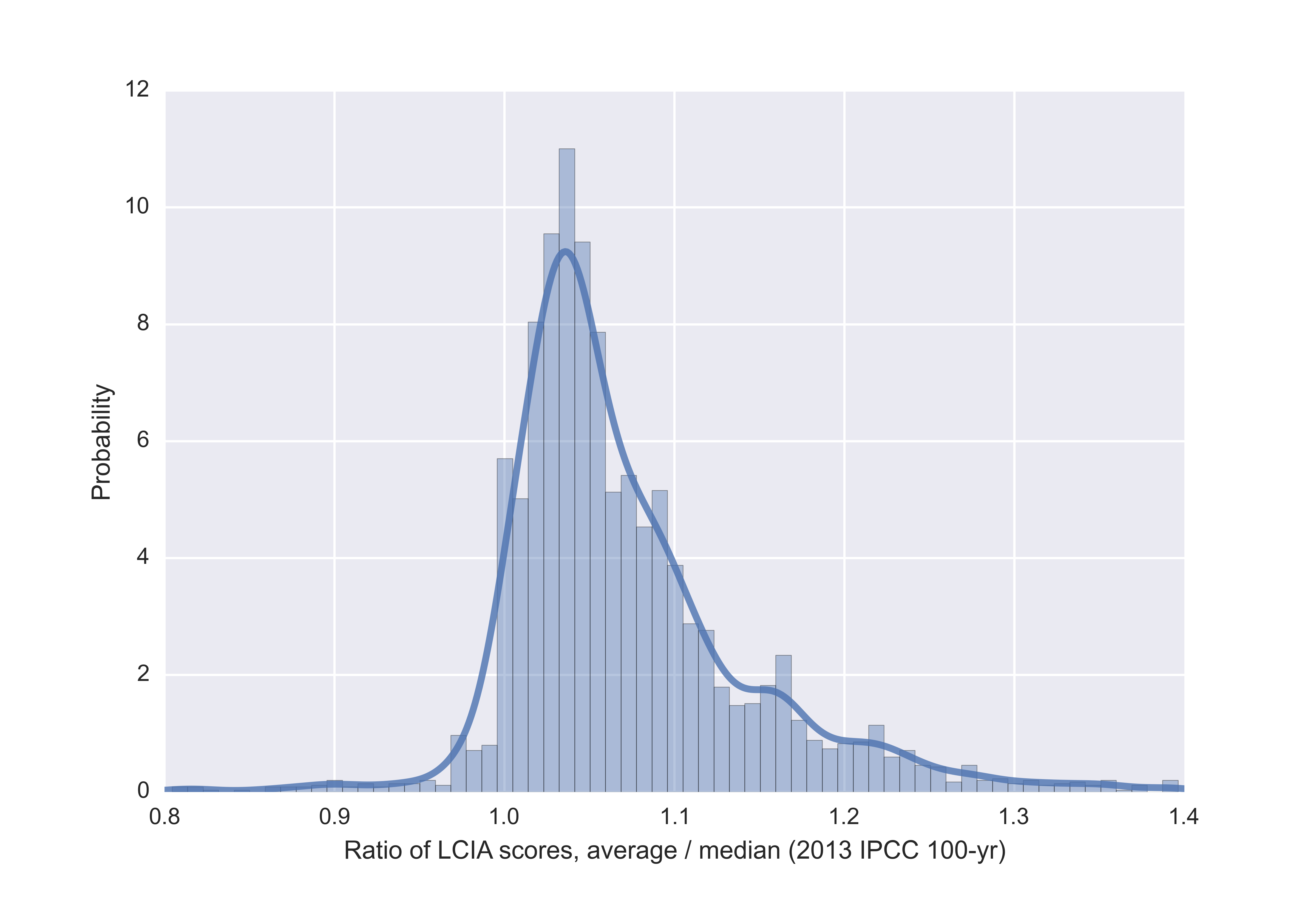
Ration of average to median LCIA scores for processes from ecoinvent 2.2.

The difference is significant - an average of 4.5% higher scores, a median of 5.3% higher scores, with some much larger differences. Is this difference a problem? The median values were chosen for good reasons, and often represent the one good data point we have in inventory datasets. I don't think we can just decide to switch from the median to average values - instead, the question is whether our one good data point represents the average or median of the population. I don't have an answer, but I think this is something that the community should think about.

Ouroboros

There is also no standard, for the best of my knowledge, on how to specify and interpret processes which consume some of their own reference product. For example, an electrical generator might need electricity to run its various pollution control equipment. If the pollution control equipment were in a separate dataset, there would be no problem in visualizing the supply chain or constructing the technosphere matrix:

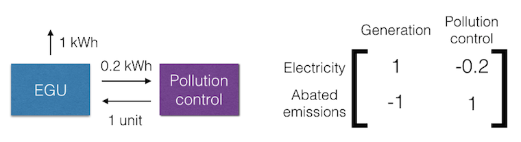
To get one kilowatt-hour of electricity, we need 1.25 units of "EGU" (activities are columns, products are rows; see What happens with a non-unitary production amount in LCA?). However, if we have a single process which consumes as an input some of its own reference product, then the situation is less clear:

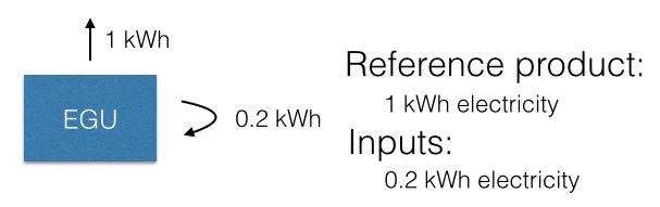
What number do we place in the technosphere matrix diagonal? It depends on whether you think the 1 kwh is the gross or net amount of reference product produced. Brightway2 uses the SciPy sparse matrix format "COO" (coordinate matrix), where duplicate entries are added together. So, in Brightway2, the value on the diagonal would be $1 - 0.2 = 0.8$ (SimaPro has the same behaviour). This is the gross production assumption, and the net production of 0.8 is the value inserted into the technosphere. The value of 0.2 represents the amount of the gross production lost to inefficiency, pollution control, etc. Note that this is not a fractional amount, but an absolute amount, and has the same units as the reference product.

In most cases, it is more convenient to scale up the activity so that it produces 1.25 kWh of gross production, with a loss of 0.25 kWh, and a net production of 1 kWh. An activity that is only 50% efficient would have a gross production of 2, a loss of 1, and a net production of 1. Having a technosphere matrix with only ones on the diagonal gives a lot of advantages.

The net production approach is consistent with how the math would work if there were two separate datasets. However, from personal communication, I know that many datasets in ecoinvent are modeled using the net production assumption. In this case, 0.2 represents the additional amount of reference product needed for to get the net production amount. In the net production assumption, the value inserted into the technosphere matrix would be:

In this case, the difference between technosphere values is not great - $0.8$ versus $ 0.8\overline{3} $. The difference between the two assumptions increases with the level of inefficiency.

The gross production assumption introduces complications - it makes it harder to build the technosphere matrix, as you can't just add numbers. But in many cases primary data sources follow this approach, and it is easier for some to understand. I personally prefer the gross production assumption, if only because it is consistent whether the activity is split into two datasets or one. The important point is that there should be clear standards for LCI datasets.

Conclusions

Although the field of life cycle assessment is well established, there are still some basic questions that need to answered in a consistent way if we want meaningful results. This blog post discussed two such standardization questions, which as far as I know are not addressed in the literature. I could be wrong - maybe there is a standard in an out-of-print SETAC document from the 90s. There are certainly more open questions, however. Before we devote all our research energy to expanding the boundaries of LCA in new directions, we should remember that our exotic constructions are only as strong as the foundations they are built upon.